CSC477 Introduction to Mobile Robotics
Week #11: Particle Filters
KF vs EKF vs PF
| Kalman Filter | Extended Kalman Filter | Particle Filter | |
|---|---|---|---|
| Dynamics model | Linear | Nonlinear | Nonlinear |
| Sensor model | Linear | Nonlinear | Nonlinear |
| Noise | Gaussian (Unimodal) | Gaussian (Unimodal) | Multimodal |
How can we represent multimodal distributions?


Idea #1: Histograms
Advantages: the higher the number of bars the better the approximation is
Disadvantages: exponential dependence on number of dimensions
Note: this approach is called the Histogram Filter. It is useful for low-dimensional systems but we will not study it in this class.
Idea #2: Function Approximation
How can we represent multimodal distributions?

Idea #1: Histograms
Advantages: the higher the number of bars the better the approximation is
Disadvantages: exponential dependence on number of dimensions
Note: this approach is called the Histogram Filter. It is useful for low-dimensional systems but we will not study it in this class.
Idea #2: Function Approximation
Idea #3: Weighted Particles \(\{(x^{[1]},w^{[1]}),...,(x^{[M]},w^{[M]})\}\)
Advantages: easy to predict/update by treating each particle as a separate hypothesis whose weight is updated.
Disadvantages: need enough particles to “cover” the distribution
How can we represent multimodal distributions?
\[\begin{align} bel(x_t) &= p(x_t|z_{0:t}, u_{0:t-1}) \\ &= \sum_{m=1}^{M} \begin{cases} w^{[m]}/W & \text{if } x_t=x_t^{[m]} \\ 0 & \text{o.w.} \end{cases} \end{align}\]
Idea #1: Histograms
Advantages: the higher the number of bars the better the approximation is
Disadvantages: exponential dependence on number of dimensions
Note: this approach is called the Histogram Filter. It is useful for low-dimensional systems but we will not study it in this class.
Idea #2: Function Approximation
Idea #3: Weighted Particles \(\{(x^{[1]},w^{[1]}),...,(x^{[M]},w^{[M]})\}\)
Advantages: easy to predict/update by treating each particle as a separate hypothesis whose weight is updated.
Disadvantages: need enough particles to “cover” the distribution
Higher density of
particles means
higher probability
mass
How can we represent multimodal distributions?
Want particles to be drawn from the belief at time t:
\[x_{t}^{[m]}\sim p(x_{t}|z_{0:t},u_{0:t-1})\]
Idea #1: Histograms
Advantages: the higher the number of bars the better the approximation is
Disadvantages: exponential dependence on number of dimensions
Note: this approach is called the Histogram Filter. It is useful for low-dimensional systems but we will not study it in this class.
Idea #2: Function Approximation
Idea #3: Weighted Particles \(\{(x^{[1]},w^{[1]}),...,(x^{[M]},w^{[M]})\}\)
Advantages: easy to predict/update by treating each particle as a separate hypothesis whose weight is updated.
Disadvantages: need enough particles to “cover” the distribution
Higher density of
particles means
higher probability
mass
Particle propagation/prediction
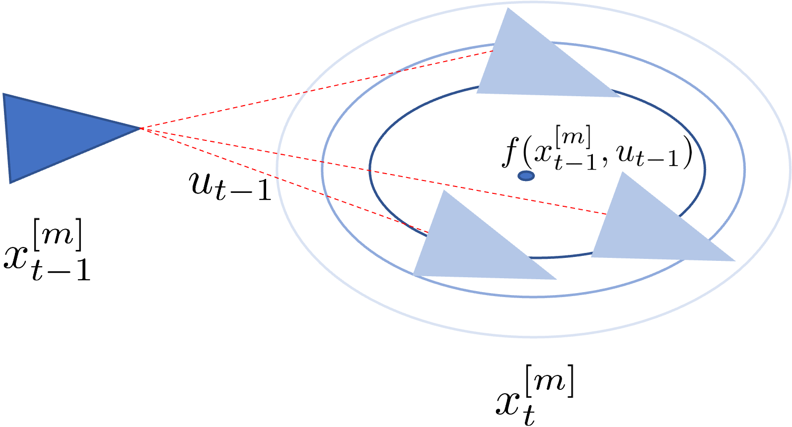
Simulate what is going to happen to the particle at the next time step by drawing a sample from the next state specified in the dynamics (a.k.a. one-step simulator)
\[x_t^{[m]} \sim p(x_t | x_{t-1}^{[m]}, u_{t-1})\]
Usually
\[\begin{aligned} x_{t}^{[m]}=f(x_{t-1}^{[m]},u_{t-1})+w_{t-1}\\ w_{t-1}\sim\mathcal{N}(0,Q) \end{aligned}\]
How to update particle weights after an observation
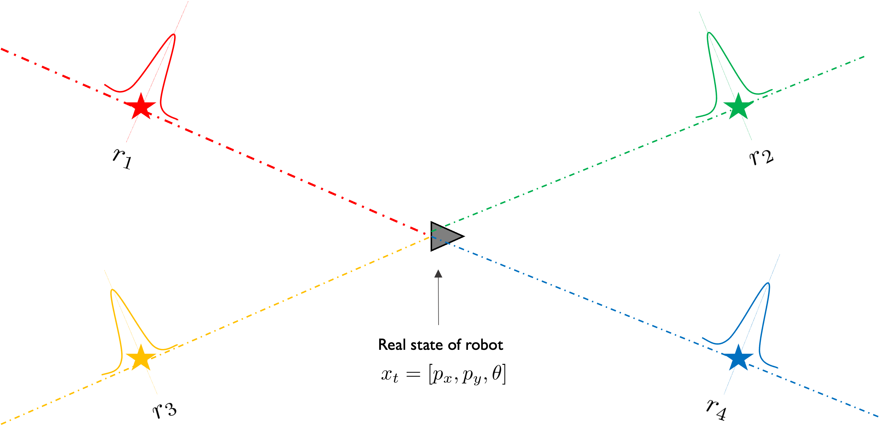
Measurement model \(z_t = h(x_t) + n_t = [r_1, r_2, r_3, r_4] + n_t\)
with \(r_i = \sqrt{(p_x - l_x^{(i)})^2 + (p_y - l_y^{(i)})^2}\) and \(n_i \sim \mathcal{N}(0, \sigma^2)\)
\[\left. \rule{0pt}{1cm} \right\} p(z_t|x_t) = \mathcal{N}(z_t; r_{1:4}, \sigma^2 \mathbb{I}_4)\]
How to update particle weights after an observation
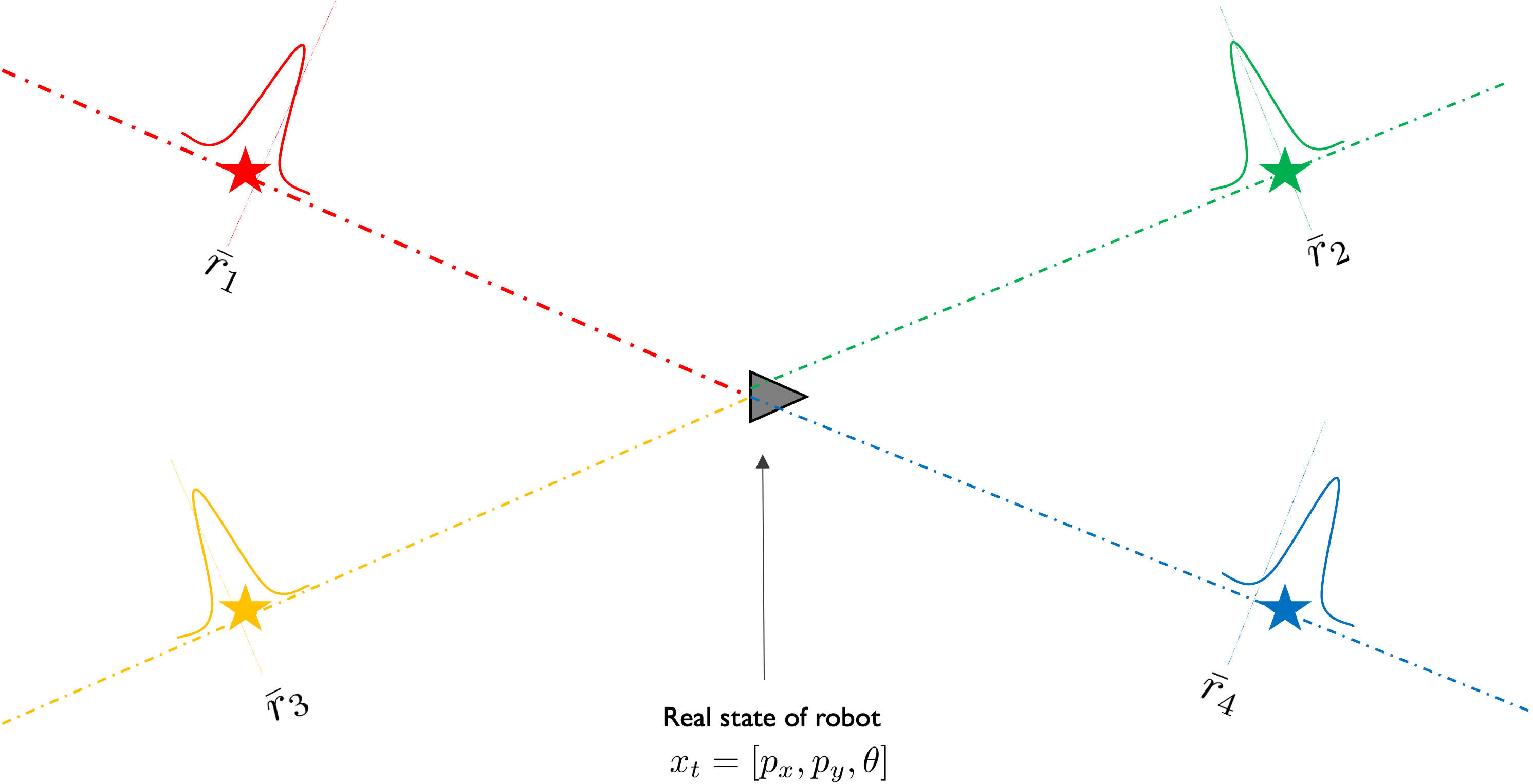
Actual measurement received: \({\bar{z}_t = [\bar{r}_1, \bar{r}_2, \bar{r}_3, \bar{r}_4]}\)
How to update particle weights after an observation
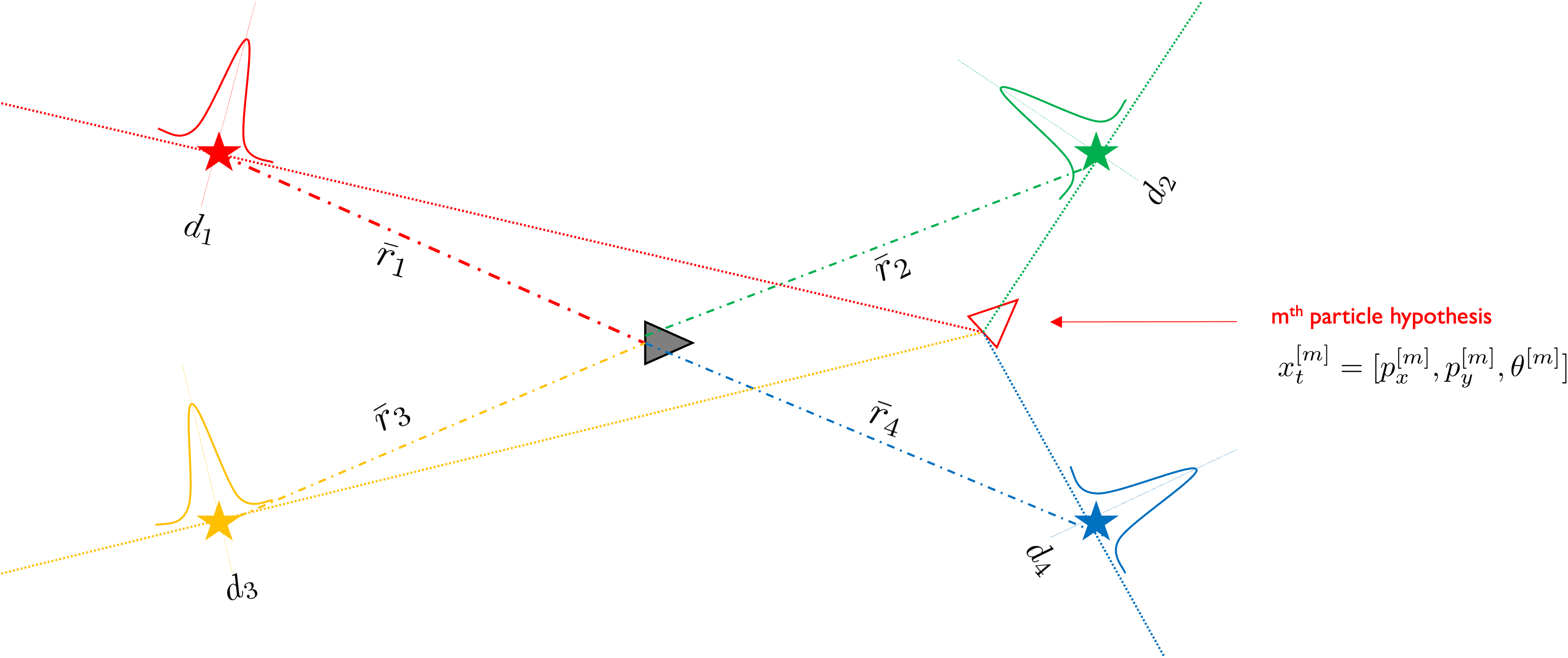
Measurement model \(z_{t}=h(x_{t}^{[m]})+n_{t}=[d_{1},d_{2},d_{3},d_{4}]+n_{t}\)
with \(d_{i}=\sqrt{(p_{x}^{[m]}-l_{x}^{(i)})^{2}+(p_{y}^{[m]}-l_{y}^{(i)})^{2}}\) and \(n_i \sim \mathcal{N}(0, \sigma^2)\)
\[\left. \rule{0pt}{1cm} \right\} p(z_t|x_t^{[m]}) = \mathcal{N}(z_t; d_{1:4}, \sigma^2 \mathbb{I}_4)\]
How to update particle weights after an observation
Q: What is the probability of the actual measurement given the state hypothesized by the particle?
A: \(p(\bar{z}_t | x_t^{[m]}) = \mathcal{N}(\bar{z}_t; d_{1:4}, \sigma^2 \mathbb{I}_4) = \eta \exp(-\|\bar{z}_t - d_{1:4}\|^2 / \sigma^2)\)
How to update particle weights after an observation
Q: What is the probability of the actual measurement given the state hypothesized by the particle?
A: \(p(\bar{z}_{t}|x_{t}^{[m]}) = \prod_{i=1}^{4} p(\bar{r}_{i}|x_{t}^{[m]}) = \prod_{i=1}^{4} \mathcal{N}(\bar{r}_{i}; d_{i}, \sigma^{2}) = \prod_{i=1}^{4} \eta \exp(-(\bar{r}_{i}-d_{i})/\sigma^{2})\)
Assuming range measurements
are conditionally independent
given state
How to update particle weights after an observation
Q: What is the probability of the actual measurement given the state hypothesized by the particle?
A: \(p(\bar{z}_{t}|x_{t}^{[m]}) = \prod_{i=1}^{4} p(\bar{r}_{i}|x_{t}^{[m]}) = \prod_{i=1}^{4} \mathcal{N}(\bar{r}_{i}; d_{i}, \sigma^{2})\)
In the figure above this probability would be low
and this particle would be unlikely.
How to update particle weights after an observation
Particle’s (unnormalized) weight \(\quad w_t^{[m]} \propto p(\bar{z}_t | x_t^{[m]})\)
See Appendix 1 for why
this choice was made
for the weight
The distribution of the particles has not been updated yet. We only updated their weights. To update the distribution of particles we need to do resampling
Sample particles with repetition/replacement,
according to their updated weights.
Resampling Particles: Algorithm #2
new_particles = []
sample r ~ Uniform[0, 1/N]
c = weights[0]
idx = 0
for n = 1…N:
\(\qquad\) u = r + (n-1)/N
\(\qquad\) while u > c:
\(\qquad\qquad\) idx = idx + 1
\(\qquad\qquad\) c = c + weights[idx]
\(\qquad\) p = particles[idx].copy()
\(\qquad\) new_particles.append(p)
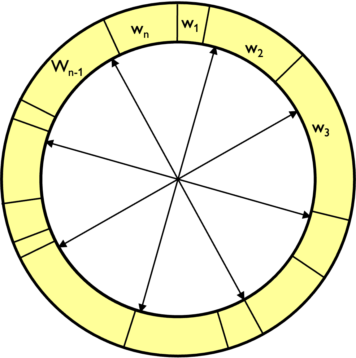
- Stochastic universal sampling
- Systematic resampling
- Linear time complexity
Particle Filter Algorithm
\[\begin{aligned} &\text{ParticleFilter}(\bar{z}_t, u_{t-1}) \\ &\qquad\bar{S}_t = \{\} \quad \bar{W}_t = \{\} \\ &\qquad\text{for particle index } m = 1...M \\ &\qquad\qquad \text{sample } x_t^{[m]} \sim p(x_t|x_{t-1}^{[m]}, u_{t-1}) \\ &\qquad\qquad w_t^{[m]} = p(\bar{z}_t|x_t^{[m]}) \\ &\qquad\qquad \bar{S}_t.\text{append}(x_t^{[m]}) \\ &\qquad\qquad \bar{W}_t.\text{append}(w_t^{[m]}) \\ \\ &\qquad S_t = \{\} \\ &\qquad\text{for particle index } m = 1...M \\ &\qquad\qquad \text{sample particle i from } \bar{S}_t \text{ with probability } \propto w_i^{[i]} \\ &\qquad\qquad S_t.\text{append}(x_t^{[m]}) \\ \\ &\quad\text{return } S_t \end{aligned}\]
 Actual observation and control received
Particle propagation/prediction:
noise needs to be added in order to make
particles differentiate from each other.
If propagation is deterministic then particles
are going to collapse to a single particle after a
few resampling steps.
Weight computation as measurement likelihood.
For each particle we compute the probability of the
actual observation given the state is at that particle.
Resampling step
Note: particle deprivation heuristics are not
shown here
Note: here we work with a fixed number of particles
but in many applications, such as localization, you could work
with a reduced number of particles after the particles have
converged to the true estimate.
Such implementations of particle filters are called adaptive. An
example is the KLD-sampling adaptive particle filter, which is
not going to be covered here.
Examples: 1D Localization

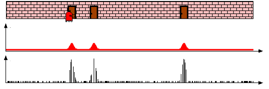
\(p(x)\)
\(p(z = \text{door} | x)\)
\(p(x|z_0 = \text{door})\)
Examples: 1D Localization

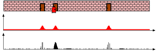
\(p(x|z_0 = \text{door}, u_0 = \text{right})\)
\(p(z = \text{door} | x)\)
\(p(x|z_0 = \text{door}, u_0 = \text{right}, z_1 = \text{door})\)
Examples: Monte Carlo Localization
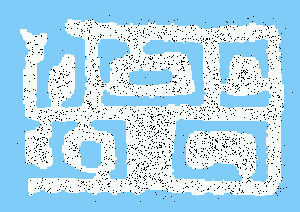
Examples: Monte Carlo Localization

After incorporating 10 ultrasound scans
Examples: Monte Carlo Localization

After incorporating 65 ultrasound scans
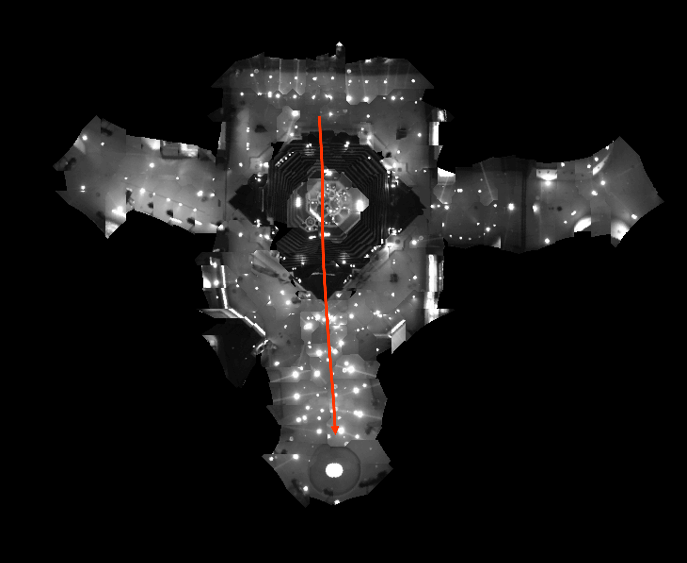
Using Ceiling Maps for Localization
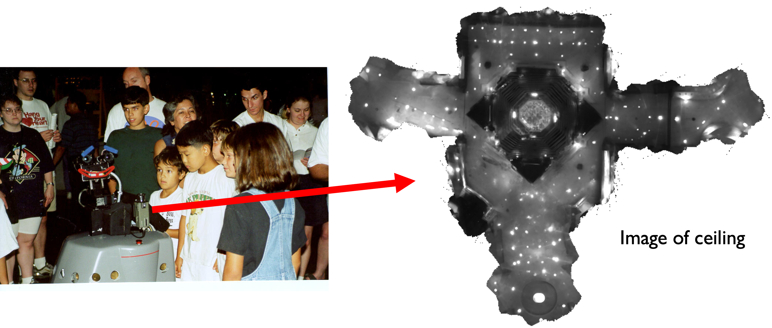
Vision-based Localization
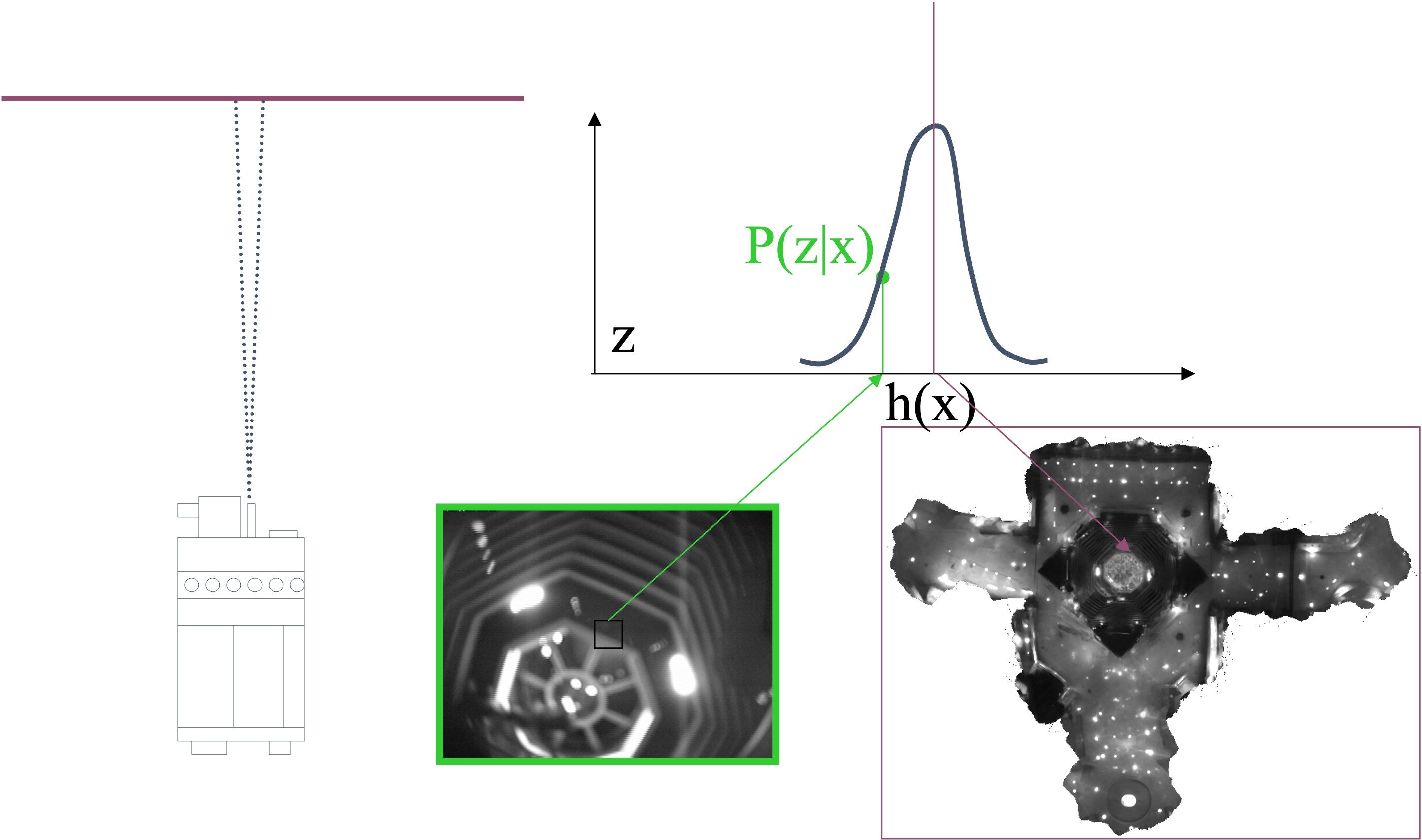
Under a Light
Measurement z:

P(z|x):
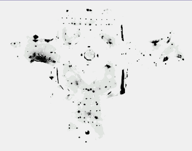
Next to a Light
Measurement z:

P(z|x):
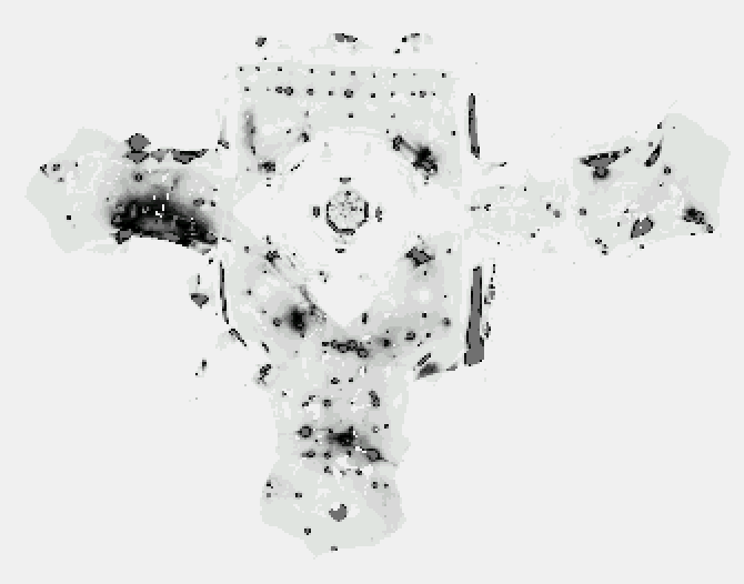
Elsewhere
Measurement z:

P(z|x):
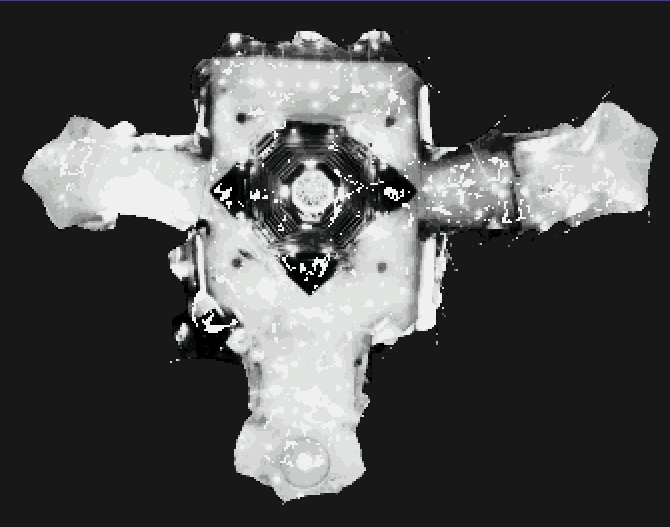
Global Localization Using Vision
Appendix 1
Why did we choose \(w_t^{[m]} \propto p(z_t|x_t^{[m]})\) as the importance weight for particle m?
Main trick: importance sampling , i.e. how to estimate properties/statistics of one distribution (f) given samples from another distribution (g)
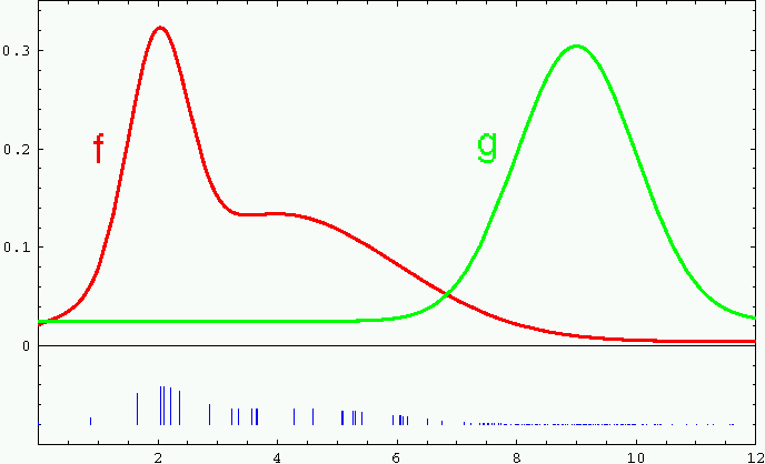
For example, suppose we want to estimate the expected value of f given only samples from g.
\[\begin{align*} \mathbb{E}_{x\sim f(x)}[x] &= \int xf(x)dx \qquad\qquad\quad \\ &= \int \frac{g(x)}{g(x)}xf(x)dx \qquad\qquad\quad \\ &= \int x\frac{f(x)}{g(x)}g(x)dx \qquad\qquad\quad \\ &= \mathbb{E}_{x\sim g(x)}\left[x\frac{f(x)}{g(x)}\right] \qquad\qquad\quad \\ &= \mathbb{E}_{x\sim g(x)}[x w(x)] \qquad\qquad\quad \end{align*}\]
Weights describe the mismatch
between the two distributions,
i.e. how to reweigh samples to
obtain statistics of f from
samples of g
Appendix 1
Why did we choose \(w_t^{[m]} \propto p(z_t|x_t^{[m]})\) as the importance weight for particle m?
Main trick: importance sampling , i.e. how to estimate properties/statistics of one distribution (f) given samples from another distribution (g)
In the case of particle filters
\(f(x_t) = p(x_t | z_{0:t}, u_{0:t-1}) = bel(x_t) \qquad g(x_t) = p(x_t | z_{0:t-1}, u_{0:t-1}) = \overline{bel}(x_t)\)
For example, suppose we want to estimate the expected value of f given only samples from g.
\[\begin{align*} \mathbb{E}_{x\sim f(x)}[x] &= \int xf(x)dx \qquad\qquad\quad \\ &= \int \frac{g(x)}{g(x)}xf(x)dx \qquad\qquad\quad \\ &= \int x\frac{f(x)}{g(x)}g(x)dx \qquad\qquad\quad \\ &= \mathbb{E}_{x\sim g(x)}\left[x\frac{f(x)}{g(x)}\right] \qquad\qquad\quad \\ &= \mathbb{E}_{x\sim g(x)}[x w(x)] \qquad\qquad\quad \end{align*}\]
Weights describe the mismatch
between the two distributions,
i.e. how to reweigh samples to
obtain statistics of f from
samples of g
Posterior belief after update \(\qquad\qquad\qquad\) Belief after propagation, before update
Appendix 1
Why did we choose \(w_t^{[m]} \propto p(z_t|x_t^{[m]})\) as the importance weight for particle m?
Main trick: importance sampling , i.e. how to estimate properties/statistics of one distribution (f) given samples from another distribution (g)
In the case of particle filters
\(f(x_t) = p(x_t | z_{0:t}, u_{0:t-1}) = bel(x_t) \qquad g(x_t) = p(x_t | z_{0:t-1}, u_{0:t-1}) = \overline{bel}(x_t)\)
For example, suppose we want to estimate the expected value of f given only samples from g.
\[\begin{align*} w(x_t^{[m]}) & = \frac{f(x_t^{[m]})}{g(x_t^{[m]})} \\ & \propto \frac{p(z_t|x_t^{[m]}) p(x_t^{[m]}|x_{t-1}^{[m]}, u_{t-1}) bel(x_{t-1}^{[m]})}{p(x_t^{[m]}|x_{t-1}^{[m]}, u_{t-1}) bel(x_t^{[m]})} \\ & \propto p(z_t|x_t^{[m]}) \end{align*}\]
Posterior belief after update \(\qquad\qquad\qquad\) Belief after propagation, before update